Feed-Forward NN

神经网络的研究和应用自上世纪四十年代以来，经历起起伏伏，到今天迎来了又一次春天。随着硬件能力的提升和可获取数据量的增加，神经网络正在打破语音识别、图像识别、自然语言处理等不同领域各自的最佳算法实践，已经或者有望成为解决多类问题的通用算法。Feed-Forward Neuron Network作为神经网络中最基础、最经典的一种，是了解神经网络的一个好起点。

Model

神经网络的基本单位是神经元（neuron），它对输入做线性加权，再应用激活函数（activation function）$$a(x)$$后输出:$$y=a(z)=a(wx+b)$$。

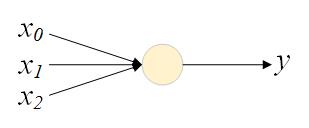
单个神经元本身就可以看作一个LR模型，已经可以很好地建模线性可分问题。而通过叠加、组合多个神经单元，可以构成更为复杂的Feed-Forward NN，进而建模更加复杂的非线性问题。

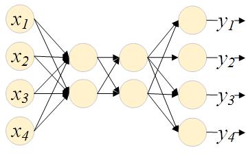
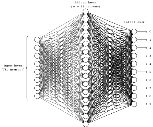
从左至右，第一层为输入层，这一层是单纯的输入示意，不做任何运算；中间两层为隐藏层，最后一层为输出层。

激活函数

常用的激活函数包括sigmod和tanh函数。他们共同的性质是对称、有界且倒数对称、有界。

在输出层，有时会应用另外一个激活函数：softmax函数。输出层应用一个softmax函数将$$z^L$$转换为一个概率分布向量：

$$ y_j^L=\frac{e^{z_j^L}}{\sum\limits_k e^{z_k^L}}

选择sigmoid还是softmax作为输出层的激活函数，需要视具体问题而定。如果多个输出不是互斥的，例如，在预测用户属性时，一个输出是性别，另一个输出是是否患病，使用sigmoid更加自然。如果多个输出之间互斥，例如，手写体识别中，每个输出分表代表一个数字，则softmax是更合适的选择。

Training

模型的训练涉及两个基本问题：代价函数定义，以及参数最优化。

代价函数：cross entropy

常用的代价函数有均方误差和cross entropy。对于常用的sigmod和tanh激活函数，均方误差代价函数会导致梯度下降缓慢(learning slowdown)，不如softmax常用，不再话下。

cross entropy作为代价函数定义如下：

$$ C=D(a^L,y)=-\frac{1}{n}\sum\limits_x\sum\limits_j y_j\log a_j^L

参数最优化：Gradient descent

Gradient descent is one of the most popular algorithms to perform optimization and by far the most common way to optimize neural networks. The architecture of neural network brings a perfect optimization method for gradient computation known as backpropagation, which leveraging chain-rule to reduce complexity significantly.

BP算法的第一个要点是巧妙地递推各层中$$C$$关于$$z$$的梯度。

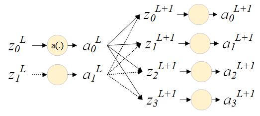
$$ \frac{\partial C}{\partial zj^l}=\sum\limits_k\frac{\partial C}{z_k^{l+1}}\frac{\partial z_k^{l+1}}{z_j^l} =\sum\limits_k\frac{\partial z_k^{l+1}}{z_j^l}\cdot\frac{\partial C}{z_k^{l+1}} =\sum\limits_k w{kj}^{l+1}\sigma'(z_j^l)\frac{\partial C}{z_k^{l+1}}

使用矩阵表示则为：

$$ \frac{\partial C}{\partial z^L}=(\frac{\partial C}{\partial a^L})\frac{\partial \sigma(z^L)}{\partial z^L}

$$ \frac{\partial C}{\partial z^l}=((W^{l+1})^T\frac{\partial C}{\partial z^{l+1}})\sigma'(z^l)

可见，每一层中$$C$$关于$$z$$的梯度可以由后一层的梯度递推而来，即误差（梯度）“从后向前层层传播”，故名Backpropagation。

BP算法的第二个要点是以$$C$$关于$$z$$的梯度为桥梁，求解$$C$$关于网络参数$$W$$和$$b$$的梯度：

$$ \frac{\partial C}{\partial b_j^l}=\frac{\partial C}{\partial z_j^l}

$$ \frac{\partial C}{\partial W_{jk}^l}={a_k^{l-1}}\frac{\partial C}{\partial {z_j^l}}

There are three variants of gradient descent, which differ in how much data we use to compute the gradient of the objective function.

Vanilla mini-batch SGD is faced with challenges. There are many algorithms trying to improve its performance, including:

Momentum
Nesterov accelerated gradient
Adagrad
Adadelta
RMSprop
Adam

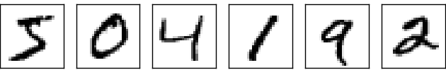
Example : mnist手写数字识别

MNIST是一个手写字符图像数据集，其中有60000训练样本，10000个测试样本。图像大小为28×28像素，像素值处于0到255之间的整数，其中，0代表黑色，255代表白色，灰度值可以通过除以255来得到。

很多论文中会将60000个训练样本分为两份：50000个样本作训练集，10000个样本作验证集（用于选择超参数，例如学习率和模型大小），我们接下来会遵循这一习惯。

用Feedforward NN来解决识别问题，输入层和输出层的维度并不难确定。问题的输入是28x28像素的灰度图像，输入层的大小即为784=28x28，每个输入是一个[0,1]的灰度值；问题的输出是0-9中的一个，输出层大小即为10，每个输出代表对答案为该数字的一种“度量”。隐藏层的维度和层数则要凭经验而定，这里，我们选择一个隐藏层，大小为15。

完整代码见Feedforward.py。BP作为整个训练算法的核心，实现上仅需要几次矩阵运算。

def backprop(self, x, y):
    """Return a tuple ``(dcdb, dcdw)`` representing the
    gradient for the cost function C_x in each layer"""
    dcdb = [np.zeros(b.shape) for b in self.biases]
    dcdw = [np.zeros(w.shape) for w in self.weights]
    # forward pass
    activation = x
    activations = [x] # list to store all the activations, layer by layer
    zs = [] # list to store all the z vectors, layer by layer
    for i, (b, w) in enumerate(zip(self.biases, self.weights)):
        z = np.dot(w, activation) + b
        zs.append(z)
        if(i == len(self.biases) - 1):
            activation = softmax(z)
        else:
            activation = sigmoid(z)
        activations.append(activation)
    # backward pass
    dcdz = (self.cost).delta(activations[-1], y)
    dcdb[-1] = dcdz
    dcdw[-1] = np.dot(dcdz, activations[-2].transpose())
    for l in xrange(2, self.num_layers):
        z = zs[-l]
        sp = sigmoid_prime(z)
        dcdz = np.dot(self.weights[-l+1].transpose(), dcdz) * sp
        dcdb[-l] = dcdz
        dcdw[-l] = np.dot(dcdz, activations[-l-1].transpose())
    return (dcdb, dcdw)

这样的一个简单实现，经过30次迭代，在validation set上可以达到97%的准确率。

Epoch 29 training complete
Cost on training data: 0.0794132821371
Accuracy on training data: 48922 / 50000
Cost on evaluation data: 0.389545105544
Accuracy on evaluation data: 9695 / 10000

Regularization

神经网络模型包含大量的参数，加上激活函数带来的非线性，有能力建模分布非常复杂的输入。所以，当模型在training_set上取得了很好的分数时，很可能是模型依赖本身很高的自由度找到了一个针对这一数据集的可行解。而数据集本身所蕴含的特征，未见得被很好地捕捉到了。这一现象称为overfitting。

overfitting发生的迹象为：模型在test_set上的准确率不再提高，但在training_set上准确率却还在提高。从实践角度来说，如果我们看到模型在test_set上的准确率不再提高，就应该停止训练。

避免或者缓解overfitting的方式有很多，例如提供更多地training data，适当减小网络大小等。除此之外，还有一些通用的方法，包括：

weight decay(L1/L2 regularization)
dropout

With L2, we can write the regularized cost function as

$$ C=C_0+\frac{\lambda}{2n}\sum\limits_w w^2

where $$C_0$$ is the original, unregularized cost function. Then The learning rule for the weights becomes:

$$ w->w-\eta\frac{dC_0}{dw}-\frac{\eta\lambda}{n}w=(1-\frac{\eta}{n})w-\eta\frac{dC_0}{dw}

The effect of weight decay is to make it so the network prefers to learn small weights. $$\lambda$$ is known as the regularization parameter. Regularization can be viewed as a way of compromising between finding small weights and minimizing the original cost function.

Why does regularization help reduce overfitting? A standard story people tell to explain what's going on is along the following lines: smaller weights are, in some sense, lower complexity, and so provide a simpler and more powerful explanation for the data, and should thus be preferred.

L2 regularization doesn't constrain the biases. Having a large bias doesn't make a neuron sensitive to its inputs in the same way as having large weights. So we don't need to worry about large biases enabling our network to learn the noise in our training data.

Another regularization approach is L1. In this approach we modify the unregularized cost function by adding the sum of the absolute values of the weights:

$$ C=C_0+\frac{\lambda}{n}\sum\limits_w|w|

Differentiating, we obtain the gradient updating rule:

$$ w->w-\frac{\eta\lambda}{n}\text{sgn}(w)-\eta\frac{dC_0}{dw}

In L2 regularization, the weights shrink by an amount which is proportional to $$w$$. In L1 regularization, when a particular weight has a large magnitude, $$|w|$$, L1 regularization shrinks the weight much less than L2 regularization does. By contrast, when $$|w|$$ is small, L1 regularization shrinks the weight much more than L2 regularization. The net result is that L1 regularization tends to concentrate the weight of the network in a relatively small number of high-importance connections, while the other weights are driven toward zero.

Dropout

Dropout和L1/L2有些不同。L1/L2是通过修改cost function来缓解overfitting，dropout则是通过修改网络结构。

每次mini-batch中，我们随机地删掉除input/output layer外hidden layer中的神经元，在删除后的新网络上计算梯度、更新参数，下一个mini-batch中随机删除另一组神经元。每次删除的节点个数占比称为dropout ratio。

由于我们每次删除的节点不同，这就像在训练大量不同的网络，然后对它们做平均。即使每个网络都会overfitting，也是以不同的方式overfitting，最终的效果是整体网络的overfitting会被减轻。

Hyper parameters

Besides weights and biases, there are many other parameters in a neural network, known as hyper parameters:

layers
neurons of each layers
initial weights
regularization
learning rate

To choose a better hyper parameter, a validation data set other than training or testing set is often applied. The approach to finding good hyper-parameters is sometimes known as the hold out, since the validation set is kept apart or "held out" from the training set.

But why we use another validation set rather than the test set? The answer is, if we set the hyper-parameters based on evaluations of the test set, it's possible we'll end up overfitting our hyper-parameters to the test set, and the performance of the network won't generalize to other data sets.

Feedforward Neuron Network